plastimatch
Synopsis
plastimatch command [options]
Description
The plastimatch executable is used for a variety of operations on either 2D or 3D images, including image registration, warping, resampling, and file format conversion. The form of the options depends upon the command given. The list of possible commands can be seen by simply typing “plastimatch” without any additional command line arguments:
$ plastimatch
plastimatch version 1.10.0
Usage: plastimatch command [options]
Commands:
 add           adjust        average       bbox          boundary
 crop          compare       compose       convert       dice
 diff          dmap          dose          drr           dvh
 fdk          fill          filter        gamma         header
 intersect     jacobian      lm-warp       mabs          mask
 maximum       ml-convert    multiply      probe         register
 resample      scale         segment       sift          stats
 synth         synth-vf      threshold     thumbnail     union
 warp          wed           xf-convert    xf-invert

For detailed usage of a specific command, type:
  plastimatch command
plastimatch add
The add command is used to add one or more images together and create an output image. The contributions of the input images can be weighted with a weight vector.
The command line usage is given as follows:
Usage: plastimatch add [options] input_file [input_file ...]
Options:
  --average        produce an output file which is the average of the
                    input files (if no weights are specified), or
                    multiply the weights by 1/n
  --output <arg>   output image
  --weight <arg>   specify a vector of weights; the images are
                    multiplied by the weight prior to adding their
                    values
Examples
To add together files 01.mha, 02.mha and 03.mha, and save the result in the file output.mha, you can run the following command:
plastimatch add --output output.mha 01.mha 02.mha 03.mha
If you wanted output.mha to be 2 * 01.mha + 0.5 * 02.mha + 0.1 * 03.mha, then you should do this:
plastimatch add \
  --output output.mha \
  --weight "2 0.5 0.1" \
  01.mha 02.mha 03.mha
plastimatch adjust
The adjust command is used to adjust the intensity values within an image. The adjustment operations available are truncation, linear scaling, histogram matching as well as global and local linear matching.
The command line usage is given as follows:
Usage: plastimatch adjust [options]
Options:
  -h, --help                    display this help message
      --hist-levels <arg>       number of histogram bins for histogram
                                 matching, default is 1024
      --hist-match <arg>        reference image for histogram matching
      --hist-points <arg>       number of match points for histogram matching,
                                 default is 10
      --hist-threshold          threshold at mean intensity (simple background
                                 exclusion) for histogram matching
      --input <arg>             input directory or filename
      --input-mask <arg>        input image mask, only affects --linear-match
                                 and --local-match
      --linear <arg>            shift and scale image intensities, provide a
                                 string with "<shift> <scale>"
      --linear-match <arg>      reference image for linear matching with mean
                                 and std
      --local-match <arg>       reference image for patch-wise shift and
                                 scale. You must specify the --patch-size
      --local-blending-off      no trilinear interpolation of shifts and
                                 scales
      --local-scale-out <arg>   filename to store pixel-wise scales
      --local-shift-out <arg>   filename to store pixel-wise shifts
      --output <arg>            output image
      --patch-size <arg>        patch size for local matching; provide 1 "n"
                                 or 3 values "nx ny nz"
      --pw-linear <arg>         a string that forms a piecewise linear map
                                 from input values to output values, of the
                                 form "in1,out1,in2,out2,..."
      --ref-mask <arg>          reference image mask, only affects
                                 --linear-match and --local-match
      --version                 display the program version
The adjust command can be used to make a piecewise linear adjustment of the image intensities. The –pw-linear option is used to create the mapping from input intensities to output intensities. The input intensities in the curve must increase from left to right in the string, but output intensities are arbitrary. Input intensities below the first pair or after the last pair are transformed by extrapolating the curve out to infinity with a slope of +1. A different slope may be specified out to positive or negative infinity by specifying the special input values of -inf and +inf. In this case, the second number in the pair is the slope of the curve, not the output intensity. You can do a simplified linear transformation of gray levels with the –linear option. For this, you need to provide a string with “<shift> <scale>”.
In addition, you can adjust the image intensities based on a reference image. With –linear-match, a linear transformation (shift and scale) is determined from mean and standard deviation of pixel values in reference and input image. If the input image feaures local intensity inconsistencies, you can choose a patch-based intensity correction using the –local-match option. Similar to –linear-match, shift and scale are computed patch-wise from mean and standard deviation. For both options, you can provide masks that specify the regions taken into account. Finally, choose –hist-match to perform histogram matching.
You can only choose one of –linear, –pw-linear, –linear-match, –local-match and –hist-match. Beware that a reference filename has to be added for matching options.
Examples
The following command will add 100 to all voxels in the image:
plastimatch adjust \
  --input infile.nrrd \
  --output outfile.nrrd \
  --pw-linear "0,100"
The following command does the same thing, but with explicit specification of the slope in the extrapolation area:
plastimatch adjust \
  --input infile.nrrd \
  --output outfile.nrrd \
  --pw-linear "-inf,1,0,100,inf,1"
The following command truncates the inputs to the range of [-1000,+1000]:
plastimatch adjust \
  --input infile.nrrd \
  --output outfile.nrrd \
  --pw-linear "-inf,0,-1000,-1000,+1000,+1000,inf,0"
The following command scales and then shifts all voxel values by 2.5 and +1000, respectively. (Use either comma or space to separate the values):
plastimatch adjust \
  --input infile.nrrd \
  --output outfile.nrrd \
  --linear "1000,2.5"
The following command matches the histogram of infile.nrrd to be similar to that of reference.nrrd:
plastimatch adjust \
  --input infile.nrrd \
  --output outfile.nrrd \
  --hist-match reference.nrrd \
  --hist-levels 1000 --hist-points 12
The following command matches mean and standard deviation of intensities in the input image to equal those of the reference image:
plastimatch adjust \
  --input infile.nrrd \
  --output outfile.nrrd \
  --linear-match reference.nrrd
The following command also matches mean and standard deviation, but calculates statistics only from inside the mask regions (note that masks are only used for statistic calculations, you would need to use plastimatch mask to reset outside values):
plastimatch adjust \
  --input infile.nrrd \
  --output outfile.nrrd \
  --linear-match reference.nrrd \
  --input-mask inmask.nrrd --ref-mask refmask.nrrd
Finally, you can apply patch-wise local intensity adjustment using the following command:
plastimatch adjust \
  --input infile.nrrd \
  --output outfile.nrrd \
  --local-match reference.nrrd \
  --patch-size "20 20 10"
The –local-match option requires the input and reference to be spatially aligned. In order to reduce the influence of background pixels at the border, you can provide foreground masks for both images (if only one mask is given, it as also used for the second image):
plastimatch adjust \
  --input infile.nrrd
  --output outfile.nrrd \
  --local-match reference.nrrd \
  --patch-size "20 20 10" \
  --input-mask inmask.nrrd \
  --ref-mask refmask.nrrd
plastimatch average
The average command is used to compute the (weighted) average of multiple input images. It is the same as the plastimatch add command, with the –average option specified. Please refer to plastimatch add for the list of command line arguments.
Example
The following command will compute the average of three input images:
plastimatch average \
  --output outfile.nrrd \
  01.mha 02.mha 03.mha
plastimatch autolabel
The autolabel command is an experimental program the uses machine learning to identify the thoracic vertibrae in a CT scan.
The command line usage is given as follows:
Usage: plastimatch autolabel [options]
Options:
  -h, --help            Display this help message
      --input <arg>     Input image filename (required)
      --network <arg>   Input trained network filename (required)
      --output <arg>    Output csv filename (required)
plastimatch boundary
The boundary command takes a binary label image as input, and generates an image of the image boundary as the output. The boundary is defined as the voxels within the label which have neighboring voxels outside the label.
The command line usage is given as follows:
Usage: plastimatch boundary [options] input_file
Required:
  --output <arg>   filename for output image
plastimatch crop
The crop command crops out a rectangular portion of the input file, and saves that portion to an output file. The command line usage is given as follows:
Usage: plastimatch crop [options]
Required:
    --input=image_in
    --output=image_out
    --voxels="x-min x-max y-min y-max z-min z-max" (integers)
The voxels are indexed starting at zero.
In other words, if the size of the image is
 ,
the x values should range between 0 and
,
the x values should range between 0 and  .
.
Example
The following command selects the region of size
 , with the first voxel of the output
image being at location (5,8,12) of the input image:
, with the first voxel of the output
image being at location (5,8,12) of the input image:
plastimatch crop \
  --input in.mha \
  --output out.mha \
  --voxels "5 14 8 17 12 21"
plastimatch compare
The compare command compares two files by subtracting one file from the other, and reporting statistics of the difference image. The two input files must have the same geometry (origin, dimensions, and voxel spacing). The command line usage is given as follows:
Usage: plastimatch compare image_in_1 image_in_2
Example
The following command subtracts synth_2 from synth_1, and reports the statistics:
$ plastimatch compare synth_1.mha synth_2.mha
MIN -558.201904 AVE 7.769664 MAX 558.680847
MAE 85.100204 MSE 18945.892578
DIF 54872 NUM 54872
The reported statistics are interpreted as follows:
MIN      Minimum value of difference image
AVE      Average value of difference image
MAX      Maximum value of difference image
MAE      Mean average value of difference image
MSE      Mean squared difference between images
DIF      Number of pixels with different intensities
NUM      Total number of voxels in the difference image
plastimatch compose
The compose command is used to compose two transforms. The command line usage is given as follows:
Usage: plastimatch compose file_1 file_2 outfile

Note:  file_1 is applied first, and then file_2.
          outfile = file_2 o file_1
          x -> x + file_2(x + file_1(x))
The transforms can be of any type, including translation, rigid, affine, itk B-spline, native B-spline, or vector fields. The output file is always a vector field.
There is a further restriction that at least one of the input files must be either a native B-spline or vector field. This restriction is required because that is how the resolution and voxel spacing of the output vector field is chosen.
Example
Suppose we want to compose a rigid transform (rigid.tfm) with a vector field (vf.mha), such that the output transform is equivalent to applying the rigid transform first, and the vector field second.
plastimatch compose rigid.tfm vf.mha composed_vf.mha
plastimatch convert
The convert command is used to convert files from one format to another format. As part of the conversion process, it can also apply (linear or deformable) geometric transforms to the input images. In fact, convert is just an alias for the warp command.
The command line usage is given as follows:
Usage: plastimatch convert [options]
Options:
 --algorithm <arg>         algorithm to use for warping, either
                            "itk" or "native", default is native
 --ctatts <arg>            ct attributes file (used by dij warper)
 --default-value <arg>     value to set for pixels with unknown
                            value, default is 0
 --dicom-with-uids <arg>   set to false to remove uids from created
                            dicom filenames, default is true
 --dif <arg>               dif file (used by dij warper)
 --dim <arg>               size of output image in voxels "x [y z]"
 --direction-cosines <arg>
                           oriention of x, y, and z axes; Specify
                            either preset value,
                            {identity,rotated-{1,2,3},sheared}, or 9
                            digit matrix string "a b c d e f g h i"
 --dose-scale <arg>        scale the dose by this value
 --fixed <arg>             fixed image (match output size to this
                            image)
 --input <arg>             input directory or filename; can be an
                            image, structure set file (cxt or
                            dicom-rt), dose file (dicom-rt,
                            monte-carlo or xio), dicom directory, or
                            xio directory
 --input-cxt <arg>         input a cxt file
 --input-dose-ast <arg>    input an astroid dose volume
 --input-dose-img <arg>    input a dose volume
 --input-dose-mc <arg>     input an monte carlo volume
 --input-dose-xio <arg>    input an xio dose volume
 --input-prefix <arg>      input a directory of structure set
                            images (one image per file)
 --input-ss-img <arg>      input a structure set image file
 --input-ss-list <arg>     input a structure set list file
                            containing names and colors
 --interpolation <arg>     interpolation to use when resampling,
                            either "nn" for nearest neighbors or
                            "linear" for tri-linear, default is
                            linear
 --metadata <arg>          patient metadata (you may use this
                            option multiple times), option written
                            as "XXXX,YYYY=string"
 --modality <arg>          modality metadata: such as {CT, MR, PT},
                            default is CT
 --origin <arg>            location of first image voxel in mm "x y
                            z"
 --output-colormap <arg>   create a colormap file that can be used
                            with 3d slicer
 --output-cxt <arg>        output a cxt-format structure set file
 --output-dicom <arg>      create a directory containing dicom and
                            dicom-rt files
 --output-dij <arg>        create a dij matrix file
 --output-dose-img <arg>   create a dose image volume
 --output-img <arg>        output image; can be mha, mhd, nii,
                            nrrd, or other format supported by ITK
 --output-labelmap <arg>   create a structure set image with each
                            voxel labeled as a single structure
 --output-pointset <arg>   create a pointset file that can be used
                            with 3d slicer
 --output-prefix <arg>     create a directory with a separate image
                            for each structure
 --output-prefix-fcsv <arg>
                           create a directory with a separate fcsv
                            pointset file for each structure
 --output-ss-img <arg>     create a structure set image which
                            allows overlapping structures
 --output-ss-list <arg>    create a structure set list file
                            containing names and colors
 --output-type <arg>       type of output image, one of {uchar,
                            short, float, ...}
 --output-vf <arg>         create a vector field from the input xf
 --output-xio <arg>        create a directory containing xio-format
                            files
 --patient-id <arg>        patient id metadata: string
 --patient-name <arg>      patient name metadata: string
 --patient-pos <arg>       patient position metadata: one of
                            {hfs,hfp,ffs,ffp}
 --prefix-format <arg>     file format of rasterized structures,
                            either "mha" or "nrrd"
 --prune-empty             delete empty structures from output
 --referenced-ct <arg>     dicom directory used to set UIDs and
                            metadata
 --series-description <arg>
                           series description metadata: string
 --simplify-perc <arg>     delete <arg> percent of the vertices
                            from output polylines
 --spacing <arg>           voxel spacing in mm "x [y z]"
 --version                 display the program version
 --xf <arg>                input transform used to warp image(s)
 --xor-contours            overlapping contours should be xor'd
                            instead of or'd
About referenced-ct
The referenced-ct option allows you to (a) create a dicom object which refers to existing objects and (b) copy metadata. The first function, referring to existing objects, uses the following logic to determine how references are made.
If the input objects contain a RTSTRUCT but not an Image (CT), the Frame Of Reference UID (0020,0052), the Series Instance UID (0020,000e) within the RT Referenced Series Sequence (3006,0014), the Referenced SOP Instance UIDs (0008,1155), and the Referenced Frame Of Reference UID (3006,0024) are all set to UIDs of the Image of the referenced-ct.
If the input objects contain a RTDOSE but not a RTSTRUCT, the Referenced Structure Set Sequence (0008,1155) is set to the UID of the RTSTRUCT of the referenced-ct.
If the input objects contain a RTDOSE but not a RTPLAN, the Referenced Structure Set Sequence (0008,1155) is set to the UID of the RTPLAN of the referenced-ct.
For the second function, the following data are copied from the referenced-ct. They are copied from the Image.
Patient Name (0010,0010)
Patient ID (0010,0020)
Examples
The first example demonstrates how to convert a DICOM volume to NRRD. The DICOM images that comprise the volume must be stored in a single directory, which for this example is called “dicom-in-dir”. Because the –output-type option was not specified, the output type will be matched to the type of the input DICOM volume. The format of the output file (NRRD) is determined from the filename extension.
plastimatch convert \
  --input dicom-in-dir \
  --output-img outfile.nrrd
This example further converts the type of the image intensities to float.
plastimatch convert \
  --input dicom-in-dir \
  --output-img outfile.nrrd \
  --output-type float
The next example shows how to resample the output image to a different geometry. The –origin option sets the position of the (center of) the first voxel of the image, the –dim option sets the number of voxels, and the –spacing option sets the distance between voxels. The units for origin and spacing are assumed to be millimeters.
plastimatch convert \
  --input dicom-in-dir \
  --output-img outfile.nrrd \
  --origin "-200 -200 -165" \
  --dim "250 250 110" \
  --spacing "2 2 2.5"
Generally speaking, it is tedious to manually specify the geometry of the output file. If you want to match the geometry of the output file with an existing file, you can do this using the –fixed option.
plastimatch convert \
  --input dicom-in-dir \
  --output-img outfile.nrrd \
  --fixed reference.nrrd
This next example shows how to convert a DICOM RT structure set file into an image using the –output-ss-img option. Because structures in DICOM RT are polylines, they are rasterized to create the image. The voxels of the output image are 32-bit integers, where the i^th bit of each integer has value one if the voxel lies with in the corresponding structure, and value zero if the voxel lies outside the structure. The structure names are stored in separate file using the –output-ss-list option.
plastimatch convert \
  --input structures.dcm \
  --output-ss-img outfile.nrrd \
  --output-ss-list outfile.txt
In the previous example, the geometry of the output file wasn’t specified. When the geometry of a DICOM RT structure set isn’t specified, it is assumed to match the geometry of the DICOM (CT, MR, etc) image associated with the contours. If the associated DICOM image is in the same directory as the structure set file, it will be found automatically. Otherwise, we have to tell plastimatch where it is located with the –referenced-ct option.
plastimatch convert \
  --input structures.dcm \
  --output-ss-img outfile.nrrd \
  --output-ss-list outfile.txt \
  --referenced-ct ../image-directory
plastimatch dice
The plastimatch dice compares binary label images using Dice coefficient, Hausdorff distance, or contour mean distance. The input images are treated as boolean, where non-zero values mean that voxel is inside of the structure and zero values mean that the voxel is outside of the structure.
The command line usage is given as follows:
Usage: plastimatch dice [options] reference-image test-image
Options:
 --all            Compute Dice, Hausdorff, and contour mean
                   distance (equivalent to --dice --hausdorff
                   --contour-mean)
 --contour-mean   Compute contour mean distance
 --dice           Compute Dice coefficient (default)
 --hausdorff      Compute Hausdorff distance and average Hausdorff
                   distance
Example
The following command computes all three statistics for mask1.mha and mask2.mha:
plastimatch dice --all mask1.mha mask2.mha
plastimatch diff
The plastimatch diff command subtracts one image from another, and saves the output as a new image. The two input files must have the same geometry (origin, dimensions, and voxel spacing).
The command line usage is given as follows:
Usage: plastimatch diff image_in_1 image_in_2 image_out
Example
The following command computes file1.nrrd minus file2.nrrd, and saves the result in outfile.nrrd:
plastimatch diff file1.nrrd file2.nrrd outfile.nrrd
plastimatch dmap
The plastimatch dmap command takes a binary label image as input, and creates a distance map image as the output. The output image has the same image geometry (origin, dimensions, voxel spacing) as the input image.
The command line usage is given as follows:
Usage: plastimatch dmap [options]
Required:
 --input <arg>        input directory or filename
 --output <arg>       output image
Optional:
 --algorithm <arg>    a string that specifies the algorithm used
                       for distance map calculation, either
                       "maurer", "danielsson", or "itk-danielsson"
                       (default is "danielsson")
 --inside-positive    voxels inside the structure should be
                       positive (by default they are negative)
 --maximum-distance <arg>
                      voxels with distances greater than this
                       number will have the distance truncated to
                       this number
 --squared-distance   return the squared distance instead of
                       distance
Example
The following command computes a distance map file dmap.nrrd from a binary labelmap image label.nrrd.:
plastimatch dmap --input label.nrrd --output dmap.nrrd
plastimatch drr
A digitally reconstructed radiograph (DRR) is a synthetic radiograph which can be generated from a computed tomography (CT) scan. It is used as a reference image for verifying the correct setup position of a patient prior to radiation treatment.
The plastimatch drr command takes a CT image as input, and generates one or more output images. The output images can be either pgm, pfm, or raw format. The command line usage is:
Usage: plastimatch drr [options] [infile]
Options:
 -i, --algorithm <arg>         Choose algorithm {exact,uniform}
     --autoscale               Automatically rescale intensity
     --autoscale-range <arg>   Range used for autoscale in form "min
                                max" (default: "0 255")
 -z, --detector-size <arg>     The physical size of the detector in
                                format "row col", in mm
 -r, --dim <arg>               The output resolution in format "row
                                col" (in mm)
 -e, --exponential             Do exponential mapping of output values
 -y, --gantry-angle <arg>      Gantry angle for image source in degrees
 -N, --gantry-angle-spacing <arg>
                               Difference in gantry angle spacing in
                                degrees
 -G, --geometry-only           Create geometry files only
 -h, --help                    display this help message
 -P, --hu-conversion <arg>     Choose HU conversion type
                                {preprocess,inline,none}
 -c, --image-center <arg>      The image center in the format "row
                                col", in pixels
 -I, --input <arg>             Input file
 -s, --intensity-scale <arg>   Scaling factor for output image
                                intensity
 -o, --isocenter <arg>         Isocenter position "x y z" in DICOM
                                coordinates (mm)
 -n, --nrm <arg>               Normal vector of detector in format "x y
                                z"
 -a, --num-angles <arg>        Generate this many images at equal
                                gantry spacing
 -O, --output <arg>            Prefix for output file(s)
 -t, --output-format <arg>     Select output format {pgm, pfm, raw}
 -S, --raytrace-details <arg>
                               Create output file with complete ray
                                trace details
     --sad <arg>               The SAD (source-axis-distance) in mm
                                (default: 1000)
     --sid <arg>               The SID (source-image-distance) in mm
                                (default: 1500)
 -w, --subwindow <arg>         Limit DRR output to a subwindow in
                                format "r1 r2 c1 c2",in pixels
 -A, --threading <arg>         Threading option {cpu,cuda,opencl}
                                (default: cpu)
     --version                 display the program version
     --vup <arg>               The vector pointing from the detector
                                center to the top row of the detector in
                                format "x y z"
An input file is required. The drr command can be used in either single image mode or rotational mode. In single image mode, you specify the complete geometry of the x-ray source and imaging panel for a single image. In rotational mode, the imaging geometry is rotated in a circular arc around the isocenter, with a fixed source to axis distance (SAD), and projection images generated at fixed angular intervals.
Examples
The following example illustrates the use of single image mode:
plastimatch drr -nrm "1 0 0" \
    -vup "0 0 1" \
    -g "1000 1500" \
    -r "1024 768" \
    -z "400 300" \
    -c "383.5 511.5" \
    -o "0 -20 -50" \
    input_file.mha
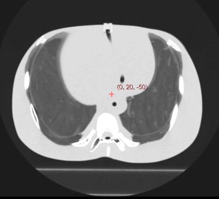
In the above example, the isocenter is chosen to be (0, -20, -50), the location marked on the CT image. The orientation of the projection image is controlled by the nrm and vup options. Using the default values of (1, 0, 0) and (0, 0, 1) yields the DRR shown on the right:
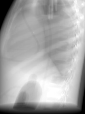
By changing the normal direction (nrm), we can choose different beam direction within an isocentric orbit. For example, an anterior-posterior (AP) DRR is generated with a normal of (0, -1, 0) as shown below:
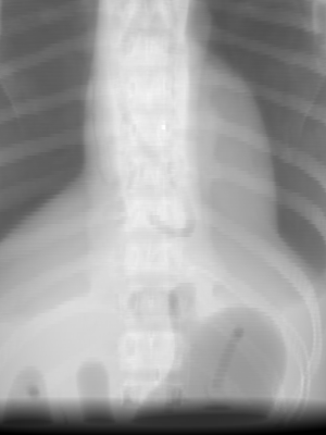
The rotation of the imaging panel is selected using the vup option. The default value of vup is (0, 0, 1), which means that the top of the panel is oriented toward the positive z direction in world coordinates. If we wanted to rotate the panel by 45 degrees counter-clockwise on our AP view, we would set vup to the (1, 0, 1) direction, as shown in the image below. Note that vup doesn’t have to be normalized.
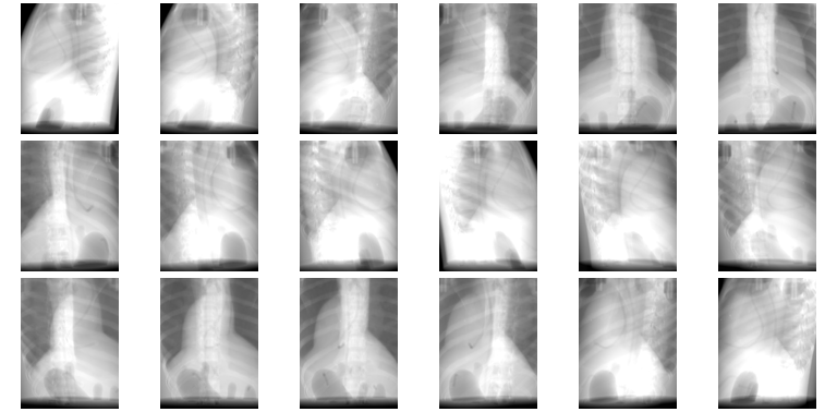
In rotional mode, multiple images are created. The source and imaging panel are assumed to rotate in a circular orbit around the isocenter. The circular orbit is performed around the Z axis, and the images are generated every -N ang degrees of the orbit. This is illustrated using the following example:
plastimatch drr -N 20 \
    -a 18 \
    -g "1000 1500" \
    -r "1024 768" \
    -z "400 300" \
    -o "0 -20 -50" \
    input_file.mha
In the above example, 18 images are generated at a 20 degree interval, as follows:
plastimatch dvh
The dvh command creates a dose value histogram (DVH) from a given dose image and structure set image. The command line usage is given as follows:
Usage: plastimatch dvh [options]
Options:
     --bin-width <arg>       specify bin width in the histogram in
                              units of Gy (default=0.5)
     --cumulative            create a cumulative DVH (this is the
                              default)
     --differential          create a differential DVH instead of a
                              cumulative DVH
     --dose-units <arg>      specify units of dose in input file as
                              either cGy as "cgy" or Gy as "gy"
                              (default="gy")
 -h, --help                  display this help message
     --input-dose <arg>      dose image file
     --input-ss-img <arg>    structure set image file
     --input-ss-list <arg>   structure set list file containing names
                              and colors
     --normalization <arg>   specify histogram values as either voxels
                              "vox" or percent "pct" (default="pct")
     --num-bins <arg>        specify number of bins in the histogram
                              (default=256)
     --output-csv <arg>      file to save dose volume histogram data in
                              csv format
     --version               display the program version
The required inputs are –input-dose, –input-ss-img, –input-ss-list, and –output-csv. The units of the input dose must be either Gy or cGy. DVH bin values will be generated for all structures found in the structure set files. The output will be generated as an ASCII csv-format spreadsheet file, readable by OpenOffice.org or Microsoft Excel.
The default is a differential (standard) histogram, rather than the cumulative DVH which is most common in radiotherapy. To create a cumulative DVH, use the –cumulative option.
The default is to create 256 bins, each with a width of 1 Gy. You can adjust these values using the –num-bins and –bin-width option.
Example
To generate a DVH for a single 2 Gy fraction, we might choose 250 bins each of width 1 cGy. If the input dose is already specified in cGy, you would use the following command:
plastimatch dvh \
  --input-ss-img structures.mha \
  --input-ss-list structures.txt \
  --input-dose dose.mha \
  --output-csv dvh.csv \
  --input-units cgy \
  --num-bins 250 \
  --bin-width 1
plastimatch fdk
The term FDK refers to the authors Feldkamp, Davis, and Kress who wrote the seminal paper “Practical cone-beam algorithm” in 1984. Their paper describes a filtered back-projection reconstruction algorithm for cone-beam geometries. The plastimatch fdk command is an implmenetation of the FDK algorithm. It takes a directory of 2D projection images as input, and generates a single 3D volume as output.
The command line usage is:
Usage: plastimatch fdk [options]
Options:
 -x, --detector-offset <arg>   The translational offset of the detector
                                "x0 y0", in pixels
 -r, --dim <arg>               The output image resolution in voxels
                                "num (num num)" (default: 256 256 100
 -f, --filter <arg>            Choice of filter {none,ramp} (default:
                                ramp)
 -X, --flavor <arg>            Implementation flavor {0,a,b,c,d}
                                (default: c)
 -h, --help                    display this help message
 -a, --image-range <arg>       Use a sub-range of available images
                                "first ((skip) last)"
 -I, --input <arg>             Input file
 -s, --intensity-scale <arg>   Scaling factor for output image
                                intensity
 -O, --output <arg>            Prefix for output file(s)
 -A, --threading <arg>         Threading option {cpu,cuda,opencl}
                                (default: cpu)
     --version                 display the program version
 -z, --volume-size <arg>       Physical size of reconstruction volume
                                "s1 s2 s3", in mm (default: 300 300 150)
The usage of the fdk command is best understood by following along with the tutorials: FDK tutorial (part 1) and FDK tutorial (part 2).
Three different formats of input files are supported. These are:
Pfm format image files with geometry txt files
Raw format image files with geometry txt files
Varian hnd files
The pfm and raw files are similar, in that they store the image as an array of 4-byte little-endian floats. The only difference is that the pfm file has a header which stores the image size, and the raw file does not.
Each pfm or raw image file must have a geometry file in the same directory with the .txt extension. For example, if you want to use image_0000.pfm in a reconstruction, you should supply another file image_0000.txt which contains the geometry. A brief description of the geometry file format is given in Projection matrix file format.
The sequence of files should be stored with the pattern:
XXXXYYYY.ZZZ
where XXXX is a prefix, YYYY is a number, and .ZZZ is the extension of a known type (either .hnd, .pfm, or .raw).
For example the following would be a good directory layout for pfm files:
Files/image_00.pfm
Files/image_00.txt
Files/image_01.pfm
Files/image_01.txt
etc...
The Varian hnd files should be stored in the original layout. For example:
Files/ProjectionInfo.xml
Files/Scan0/Proj_0000.hnd
Files/Scan0/Proj_0001.hnd
etc...
No geometry txt files are needed to reconstruct from Varian hnd format.
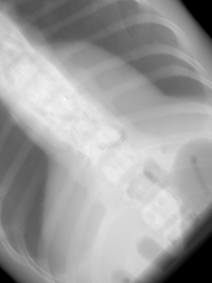
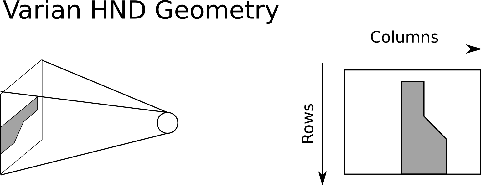
By default, when you generate a DRR, the image is oriented as if the virtual x-ray source were a camera. That means that for a right lateral film, the columns of the image go from inf to sup, and the rows go from ant to post. The Varian OBI system produces HND files, which are oriented differently. For a right lateral film, the columns of the HND images go from ant to post, and the rows go from sup to inf. An illustration of this idea is shown in the figure below.
plastimatch fill
The fill command is used to fill an image region with a constant intensity. The region filled is defined by a mask file, with voxels with non-zero intensity in the mask image being filled.
The command line usage is given as follows:
Usage: plastimatch fill [options]
Options:
  --input <arg>         input directory or filename; can be an image
                         or dicom directory
  --mask <arg>          input filename for mask image
  --mask-value <arg>    value to set for pixels within mask (for
                         "fill"), or outside of mask (for "mask"
  --output <arg>        output filename (for image file) or directory
                         (for dicom)
  --output-format <arg> arg should be "dicom" for dicom output
  --output-type <arg>   type of output image, one of {uchar, short,
                         float, ...}
Examples
Suppose we have a file prostate.nrrd which is zero outside of the prostate, and non-zero inside of the prostate. We can fill the prostate with an intensity of 1000, while leaving non-prostate areas with their original intensity, using the following command.
plastimatch fill \
  --input infile.nrrd \
  --output outfile.nrrd \
  --mask-value 1000 \
  --mask prostate.nrrd
plastimatch filter
The filter command applies a filter to an input image, and creates a filtered image as its output. The filter can be either built-in, or custom.
The command line usage is given as follows:
Usage: plastimatch filter [options] input_image
Options:
 --gabor-k-fib <arg>     choose gabor direction at index i within
                          fibonacci spiral of length n; specified as
                          "i n" where i and n are integers, and i is
                          between 0 and n-1
 --gauss-width <arg>     the width (in mm) of a uniform Gaussian
                          smoothing filter
 --kernel <arg>          kernel image filename
 --output <arg>          output image filename
 --output-kernel <arg>   output kernel filename
 --pattern <arg>         filter type: {gabor, gauss, kernel},
                          default is gauss
The built-in filters supported are “gabor” and “gauss”. For a Gaussian, the width of the Gaussian can be controlled using the –gauss-width option. The Gabor filter is currently limited to automatic selection of filter directions, which are spaced quasi-uniformly on the unit sphere. Custom filters are specified by supplying a kernel file, which is convolved with the image.
Example
The following command will generate a filtered image from the first gabor filter within a bank of 10 filters.:
plastimatch filter --pattern gabor Testing/rect-1.mha \
  --gabor-k-fib "0 5" --output g-05.mha
plastimatch gamma
The gamma command compares two images using the so-called gamma criterion. The gamma criterion specifies that images are similar at a givel location within a reference image if there exists a voxel with similar intensity nearby in the comparison image. Both local gamma and global gamma can be performed using this command.
The command line usage is given as follows:
Usage: plastimatch gamma [options] image_1 image_2
Options:
 --analysis-threshold <arg>
     Analysis threshold for dose in float (for
      example, input 0.1 to apply 10% of the
      reference dose). The final threshold dose
      (Gy) is calculated by multiplying this
      value and a given reference dose (or
      maximum dose if not given). (default is
      0.1)
 --compute-full-region    With this option, full gamma map will be
      generated over the entire image region
      (even for low-dose region). It is
      recommended not to use this option to
      speed up the computation. It has no
      effect on gamma pass-rate.
 --dose-tolerance <arg>   The scaling coefficient for dose
      difference. (e.g. put 0.02 if you want to
      apply 2% dose difference criterion)
      (default is 0.03)
 --dta-tolerance <arg>    The distance-to-agreement (DTA) scaling
      coefficient in mm (default is 3)
 --gamma-max <arg>        The maximum value of gamma to compute;
      smaller values run faster (default is
      2.0)
 --inherent-resample <arg>
     Spacing value in [mm]. The reference
      image itself will be resampled by this
      value (Note: resampling compare-image to
      ref-image is inherent already). If arg <
      0, this option is disabled. (default is
      -1.0)
 --interp-search          With this option, smart interpolation
      search will be used in points near the
      reference point. This will eliminate the
      needs of fine resampling. However, it
      will take longer time to compute.
 --local-gamma            With this option, dose difference is
      calculated based on local dose
      difference. Otherwise, a given reference
      dose will be used, which is called
      global-gamma.
 --output <arg>           Output image
 --output-failmap <arg>   File path for binary gamma evaluation
      result.
 --output-text <arg>      Text file path for gamma evaluation
      result.
 --reference-dose <arg>   The prescription dose (Gy) used to
      compute dose tolerance; if not specified,
      then maximum dose in reference volume is
      used
 --resample-nn            With this option, Nearest Neighbor will
      be used instead of linear interpolation
      in resampling the compare-image to the
      reference image. Not recommended for
      better results.
Example
A gamma image is produced from two input images using the default parameters. This will be a global gamma, using maximum intensity of the reference image as the gamma normalization value.:
plastimatch gamma --output gamma.mha \
  reference-image.mha compare-image.mha
plastimatch header
The header command is used to display simple properties about the volume, such as the image data type and image geometry.
The command line usage is given as follows:
Usage: plastimatch header [options] input_file [input_file ...]
Options:
 -h, --help      display this help message
     --version   display the program version
Example
We can display the geometry of any supported file type, such as mha, nrrd, or dicom. We can run the command as follows:
$ plastimatch header input.mha
Type = float
Planes = 1
Origin = -180 -180 -167.75
Size = 512 512 120
Spacing = 0.7031 0.7031 2.5
Direction = 1 0 0 0 1 0 0 0 1
From the header information, we see that the image has 120 slices, and each slice is 512 x 512 pixels. The slice spacing is 2.5 mm, and the in-plane pixel spacing is 0.7031 mm.
plastimatch jacobian
The jacobian command computes the Jacobian determinant of a vector field. Either a Jacobian determinant image, or its summary statistics, can be computed.
The command line usage is given as follows:
Usage: plastimatch jacobian [options]
Options:
  --input <arg>          input directory or filename of image
  --output-img <arg>     output image; can be mha, mhd, nii, nrrd,
                          or other format supported by ITK
  --output-stats <arg>   output stats file; .txt format
Example
To create a Jacobian determinant image from a vector field file vf.mha, run the following:
plastimatch jacobian \
  --input vf.mha --output-img vf_jac.mha
plastimatch lm-warp
The plastimatch lm-warp command performs deformable registration by matching corresponding point landmarks on the fixed and moving images.
The command line usage is given as follows:
Usage: plastimatch lm-warp [options]
Options:
 -a, --algorithm <arg>         RBF warping algorithm
                                {tps,gauss,wendland}
 -d, --default-value <arg>     Value to set for pixels with unknown
                                value
     --dim <arg>               Size of output image in voxels "x [y z]"
 -F, --fixed <arg>             Fixed image (match output size to this
                                image)
 -f, --fixed-landmarks <arg>   Input fixed landmarks
 -h, --help                    display this help message
 -I, --input-image <arg>       Input image to warp
 -v, --input-vf <arg>          Input vector field (applied prior to
                                landmark warping)
 -m, --moving-landmarks <arg>
                               Output moving landmarks
 -N, --numclusters <arg>       Number of clusters of landmarks
     --origin <arg>            Location of first image voxel in mm "x y
                                z"
 -O, --output-image <arg>      Output warped image
 -L, --output-landmarks <arg>
                               Output warped landmarks
 -V, --output-vf <arg>         Output vector field
 -r, --radius <arg>            Radius of radial basis function (in mm)
     --spacing <arg>           Voxel spacing in mm "x [y z]"
 -Y, --stiffness <arg>         Young modulus (default = 0.0)
     --version                 display the program version
Options “-a”, “-r”, “-Y”, “-d” are set by default to:
-a=gauss          Gaussian RBFs with infinite support
-r=50.0           Gaussian width 50 mm
-Y=0.0            No regularization of vector field
-d=-1000          Air
You may want to choose different algorithm:
-a=tps            Thin-plate splines (for global registration)
-a=wendland       Wendland RBFs with compact support (for
                   local registration)
In the case of Wendland RBFs “-r” option sets the radius of support.
Regularization of vector field is available for “gauss” and “wendland” algorithms. To regularize the output vector field increase “-Y” to ‘0.1’ and up with increment ‘0.1’.
Example
To create a vector field from coresponding landmarks in fixed.fcsv and moving.fcs using Gaussian radial basis functions, do the following:
plastimatch lm-warp \
    --output-vf vf.nrrd \
    --fixed-landmarks fixed.fcsv --moving-landmarks moving.fcsv
plastimatch mabs
The mabs command performs a multi-atlas based segmentation (MABS) operation. The command can operate in one of several training mode, or in segmentation mode.
The command line usage is given as follows:
Usage: plastimatch mabs [options] command_file
Options:
  --atlas-selection         run just atlas selection
  --convert                 pre-process atlas
  --output <arg>            output (non-dicom) directory when doing
                             a segmentation
  --output-dicom <arg>      output dicom directory when doing a
                             segmentation
  --pre-align               pre-process atlas
  --segment <arg>           use mabs to segment the specified image
                             or directory
  --train                   perform full training to find the best
                             registration and segmentation parameters
  --train-atlas-selection   run just train atlas selection
  --train-registration      perform limited training to find the
                             best registration parameters only
Prior to running the mabs command, you must create a configuration file, and you must arrange your training data into the proper directory format. For a complete description of the command file syntax and usage examples, please refer to the Image segmentation (MABS) guidebook and the Image segmentation (MABS) command file reference.
plastimatch mask
The mask command is used to fill an image region with a constant intensity. The region filled is defined by a mask file, with voxels with zero intensity in the mask image being filled. Thus, it is the inverse of the fill command.
The command line usage is given as follows:
Usage: plastimatch mask [options]
Options:
  --input <arg>           input directory or filename; can be an
                           image or dicom directory
  --mask <arg>            input filename for mask image
  --mask-value <arg>      value to set for pixels within mask (for
                           "fill"), or outside of mask (for "mask"
  --output <arg>          output filename (for image file) or
                           directory (for dicom)
  --output-format <arg>   arg should be "dicom" for dicom output
  --output-type <arg>     type of output image, one of {uchar, short,
                           float, ...}
Examples
Suppose we have a file called patient.nrrd, which is zero outside of the patient, and non-zero inside the patient. If we want to fill in the area outside of the patient with value -1000, we use the following command.
plastimatch mask \
  --input infile.nrrd \
  --output outfile.nrrd \
  --negate-mask \
  --mask-value -1000 \
  --mask patient.nrrd
plastimatch ml-convert
To be written.
plastimatch probe
The plastimatch probe command is used to examine the image intensity or vector field displacement at one or more positions within a volume. The probe positions can be specified in world coordinates (in mm), using the –location option, or as image indices using the –index option. The locations or indices are linearly interpolated if they lie between voxels.
The command line usage is given as follows:
Usage: plastimatch probe [options] file
Options:
 -i, --index <arg>      List of voxel indices, such as
                         "i j k;i j k;..."
 -l, --location <arg>   List of spatial locations, such as
                         "i j k;i j k;..."
The command will output one line for each probe requested. Each output line includes the following fields.:
PROBE#        The probe number, starting with zero
INDEX         The (fractional) position of the probe as a voxel index
LOC           The position of the probe in world coordinates
VALUE         The intensity (for volumes) or displacement
               (for vector fields)
Example
We use the index option to see an image intensity at coordinate (2,3,4), and the location option to see image intensities at two different locations:
plastimatch probe \
   --index "2 3 4" \
   --location "0 0 0; 0.5 0.5 0.5" \
   infile.nrrd
The output will include three probe results. Each probe shows the probe index, voxel index, voxel location, and intensity.
0:    2.00,    3.00,    4.00;  -22.37,  -21.05,  -19.74; -998.725891
1:   19.00,   19.00,   19.00;    0.00,    0.00,    0.00; -0.000197
2:   19.38,   19.38,   19.38;    0.50,    0.50,    0.50; -9.793450
plastimatch register
The plastimatch register command is used to peform linear or deformable registration of two images. The command line usage is given as follows:
Usage: plastimatch register command_file
The command file is an ordinary text file, which contains a single global section and one or more stages sections. The global section begins with a line containing only the string “[GLOBAL]”, and each stage begins with a line containing the string “[STAGE]”.
The global section is used to set input files, output files, and global parameters, while the each stage section defines a sequential stage of processing. For a complete description of the command file syntax, please refer to the Image registration command file reference.
Examples
If you want to register image_2.mha to match image_1.mha using B-spline registration, create a command file like this:
# command_file.txt
[GLOBAL]
fixed=image_1.mha
moving=image_2.mha
img_out=warped_2.mha
xform_out=bspline_coefficients.txt

[STAGE]
xform=bspline
impl=plastimatch
threading=openmp
max_its=30
regularization_lambda=0.005
grid_spac=100 100 100
res=4 4 2
Then, run the registration like this:
plastimatch register command_file.txt
The above example only performs a single registration stage. If you want to do multi-stage registration, use multiple [STAGE] sections. Like this:
# command_file.txt
[GLOBAL]
fixed=image_1.mha
moving=image_2.mha
img_out=warped_2.mha
xform_out=bspline_coefficients.txt

[STAGE]
xform=bspline
impl=plastimatch
threading=openmp
max_its=30
regularization_lambda=0.005
grid_spac=100 100 100
res=4 4 2

[STAGE]
max_its=30
grid_spac=80 80 80
res=2 2 1

[STAGE]
max_its=30
grid_spac=60 60 60
res=1 1 1
For more examples, please refer to the Image registration guidebook.
plastimatch resample
The resample command can be used to change the geometry of an image.
The command line usage is given as follows:
Usage: plastimatch resample [options]
Options:
    --default-value <arg>   value to set for pixels with unknown value,
                             default is 0
    --dim <arg>             size of output image in voxels "x [y z]"
    --direction-cosines <arg>
                            oriention of x, y, and z axes; Specify either
                             preset value,
                             {identity,rotated-{1,2,3},sheared}, or 9 digit
                             matrix string "a b c d e f g h i"
-F, --fixed <arg>           fixed image (match output size to this image)
-h, --help                  display this help message
    --input <arg>           input directory or filename; can be an image or
                             vector field
    --interpolation <arg>   interpolation type, either "nn" or "linear",
                             default is linear
    --origin <arg>          location of first image voxel in mm "x y z"
    --output <arg>          output image or vector field
    --output-type <arg>     type of output image, one of {uchar, short,
                             float, ...}
    --spacing <arg>         voxel spacing in mm "x [y z]"
    --subsample <arg>       bin voxels together at integer subsampling rate
                             "x [y z]"
    --version               display the program version
Example
We can use the –subsample option to bin an integer number of voxels to a single voxel. So for example, if we want to bin a cube of size 3x3x1 voxels to a single voxel, we would do the following.
plastimatch resample \
  --input infile.nrrd \
  --output outfile.nrrd \
  --subsample "3 3 1"
plastimatch scale
The scale command scales an image or vector field by multiplying each voxel by a constant value.
The command line usage is given as follows:
Usage: plastimatch scale [options] input_file
Options:
  --output <arg>   filename for output image or vector field
  --weight <arg>   scale the input image or vector field by this
                    value (float)
Example
This command creates an output file with image intensity (or voxel length) twice as large as the input values:
plastimatch scale --output output.mha --weight 2.0 input.mha
plastimatch segment
The segment command does simple threshold-based semgentation. The command line usage is given as follows:
Usage: plastimatch segment [options]
Options:
  -h, --help                    Display this help message
      --input <arg>             Input image filename (required)
      --lower-threshold <arg>   Lower threshold (include voxels
                                 above this value)
      --output-dicom <arg>      Output dicom directory (for RTSTRUCT)
      --output-img <arg>        Output image filename
      --upper-threshold <arg>   Upper threshold (include voxels
                                 below this value)
Example
Suppose we have a CT image of a water tank, and we wish to create an image which has ones where there is water, and zeros where there is air. Then we could do this:
plastimatch segment \
  --input water.mha \
  --output-img water-label.mha \
  --lower-threshold -500
If we wanted instead to create a DICOM-RT structure set, we should specify a DICOM image as the input. This will allow plastimatch to create the DICOM-RT with the correct patient name, patient id, and UIDs. The output file will be called “ss.dcm”.
plastimatch segment \
  --input water_dicom \
  --output-dicom water_dicom \
  --lower-threshold -500
plastimatch stats
The plastimatch stats command displays a few basic statistics about the image onto the screen.
The command line usage is given as follows:
Usage: plastimatch stats file [file ...]
The input files can be either 2D projection images, 3D volumes, or 3D vector fields.
Example
The following command displays statistics for the 3D volume synth_1.mha.
$ plastimatch stats synth_1.mha
MIN -999.915161 AVE -878.686035 MAX 0.000000 NUM 54872
The reported statistics are interpreted as follows:
MIN      Minimum intensity in image
AVE      Average intensity in image
MAX      Maximum intensity in image
NUM      Number of voxels in image
Example
The following command displays statistics for the 3D vector field vf.mha:
$ plastimatch stats vf.mha
Min:            0.000     -0.119     -0.119
Mean:          13.200      0.593      0.593
Max:           21.250      1.488      1.488
Mean abs:      13.200      0.594      0.594
Energy: MINDIL -6.79 MAXDIL 0.166 MAXSTRAIN 41.576 TOTSTRAIN 70849
Min dilation at: (29 19 19)
Jacobian: MINJAC -6.32835 MAXJAC 1.15443 MINABSJAC 0.360538
Min abs jacobian at: (28 36 36)
Second derivatives: MINSECDER 0 MAXSECDER 388.82 TOTSECDER 669219
  INTSECDER 1.524e+06
Max second derivative: (29 36 36)
The rows corresponding to “Min, Mean, Max, and Mean abs” each have three numbers, which correspond to the x, y, and z coordinates. Therefore, they compute these statistics for each vector direction separately.
The remaining statistics are described as follows:
MINDIL        Minimum dilation
MAXDIL        Maximum dilation
MAXSTRAIN     Maximum strain
TOTSTRAIN     Total strain
MINJAC        Minimum Jacobian
MAXJAC        Maximum Jacobian
MINABSJAC     Minimum absolute Jacobian
MINSECDER     Minimum second derivative
MAXSECDER     Maximum second derivative
TOTSECDER     Total second derivative
INTSECDER     Integral second derivative
plastimatch synth
The synth command creates a synthetic image. The following kinds of images can be created, by specifying the appropriate –pattern option. Each of these patterns come with a synthetic structure set and synthetic dose which can be used for testing.
donut – a donut shaped structure
gauss – a Gaussian blur
grid – a 3D grid
lung – a synthetic lung with a tumor
rect – a uniform rectangle within a uniform background
sphere – a uniform sphere within a uniform background
xramp – an image that linearly varies intensities in the x direction
yramp – an image that linearly varies intensities in the y direction
zramp – an image that linearly varies intensities in the z direction
The command line usage is given as follows:
Usage: plastimatch synth [options]
Options:
 --background <arg>        intensity of background region
 --cylinder-center <arg>   location of cylinder center in mm "x [y
                            z]"
 --cylinder-radius <arg>   size of cylinder in mm "x [y z]"
 --dicom-with-uids <arg>   set to false to remove uids from created
                            dicom filenames, default is true
 --dim <arg>               size of output image in voxels "x [y z]"
 --direction-cosines <arg>
                           oriention of x, y, and z axes; Specify
                            either preset value,
                            {identity,rotated-{1,2,3},sheared}, or 9
                            digit matrix string "a b c d e f g h i"
 --donut-center <arg>      location of donut center in mm "x [y z]"
 --donut-radius <arg>      size of donut in mm "x [y z]"
 --donut-rings <arg>       number of donut rings (2 rings for
                            traditional donut)
 --dose-center <arg>       location of dose center in mm "x y z"
 --dose-size <arg>         dimensions of dose aperture in mm "x [y
                            z]", or locations of rectangle corners
                            in mm "x1 x2 y1 y2 z1 z2"
 --fixed <arg>             fixed image (match output size to this
                            image)
 --foreground <arg>        intensity of foreground region
 --gabor-k-fib <arg>       choose gabor direction at index i within
                            fibonacci spiral of length n; specified
                            as "i n" where i and n are integers, and
                            i is between 0 and n-1
 --gauss-center <arg>      location of Gaussian center in mm "x [y
                            z]"
 --gauss-std <arg>         width of Gaussian in mm "x [y z]"
 --grid-pattern <arg>      grid pattern spacing in voxels "x [y z]"
 --input <arg>             input image (add synthetic pattern onto
                            existing image)
 --lung-tumor-pos <arg>    position of tumor in mm "z" or "x y z"
 --metadata <arg>          patient metadata (you may use this
                            option multiple times)
 --noise-mean <arg>        mean intensity of gaussian noise
 --noise-std <arg>         standard deviation of gaussian noise
 --origin <arg>            location of first image voxel in mm "x y
                            z"
 --output <arg>            output filename
 --output-dicom <arg>      output dicom directory
 --output-dose-img <arg>   filename for output dose image
 --output-ss-img <arg>     filename for output structure set image
 --output-ss-list <arg>    filename for output file containing
                            structure names
 --output-type <arg>       data type for output image: {uchar,
                            short, ushort, ulong, float}, default is
                            float
 --patient-id <arg>        patient id metadata: string
 --patient-name <arg>      patient name metadata: string
 --patient-pos <arg>       patient position metadata: one of
                            {hfs,hfp,ffs,ffp}
 --pattern <arg>           synthetic pattern to create: {cylinder,
                            donut, dose, gabor, gauss, grid, lung,
                            noise, rect, sphere, xramp, yramp,
                            zramp}, default is gauss
 --penumbra <arg>          width of dose penumbra in mm
 --rect-size <arg>         width of rectangle in mm "x [y z]", or
                            locations of rectangle corners in mm "x1
                            x2 y1 y2 z1 z2"
 --spacing <arg>           voxel spacing in mm "x [y z]"
 --sphere-center <arg>     location of sphere center in mm "x y z"
 --sphere-radius <arg>     radius of sphere in mm "x [y z]"
 --volume-size <arg>       size of output image in mm "x [y z]"
Examples
Create a cubic water phantom 30 x 30 x 40 cm with zero position at the center of the water surface:
plastimatch synth \
  --pattern rect \
  --output water_tank.mha \
  --rect-size "-150 150 0 400 -150 150" \
  --origin "-245.5 245.5 -49.5 449.5 -149.5 149.5" \
  --spacing "1 1 1" \
  --dim "500 500 300"
Create lung phantoms with two different tumor positions, and output to dicom:
plastimatch synth \
  --pattern lung \
  --output-dicom lung_inhale \
  --lung-tumor-pos "0 0 10"
plastimatch synth \
  --pattern lung \
  --output-dicom lung_exhale \
  --lung-tumor-pos "0 0 -10"
plastimatch synth-vf
The synth-vf command creates a synthetic vector field. The following kinds of vector fields can be created, by specifying the appropriate option.
gauss – a gaussian warp
radial – a radial expansion or contraction
translation – a uniform translation
zero – a vector field that is zero everywhere
The command line usage is given as follows:
Usage: plastimatch synth-vf [options]
Options:
 --dim <arg>             size of output image in voxels "x [y z]"
 --direction-cosines <arg>
                         oriention of x, y, and z axes; Specify
                          either preset value, {identity,
                          rotated-{1,2,3}, sheared}, or 9 digit
                          matrix string "a b c d e f g h i"
 --fixed <arg>           An input image used to set the size of the
                          output
 --gauss-center <arg>    location of center of gaussian warp "x [y
                          z]"
 --gauss-mag <arg>       displacment magnitude for gaussian warp in
                          mm "x [y z]"
 --gauss-std <arg>       width of gaussian std in mm "x [y z]"
 --origin <arg>          location of first image voxel in mm "x y
                          z"
 --output <arg>          output filename
 --radial-center <arg>   location of center of radial warp "x [y
                          z]"
 --radial-mag <arg>      displacement magnitude for radial warp in
                          mm "x [y z]"
 --spacing <arg>         voxel spacing in mm "x [y z]"
 --volume-size <arg>     size of output image in mm "x [y z]"
 --xf-gauss              gaussian warp
 --xf-radial             radial expansion (or contraction)
 --xf-trans <arg>        uniform translation in mm "x y z"
 --xf-zero               Null transform
plastimatch threshold
The threshold command creates a binary labelmap image from an input intensity image.
The command line usage is given as follows:
Usage: plastimatch threshold [options]
Options:
    --above <arg>    value above which output has value high
    --below <arg>    value below which output has value high
-h, --help           display this help message
    --input <arg>    input directory or filename
    --output <arg>   output image
    --range <arg>    a string that forms a list of threshold ranges of the
                      form "r1-lo,r1-hi,r2-lo,r2-hi,...", such that voxels
                      with intensities within any of the ranges
                      ([r1-lo,r1-hi], [r2-lo,r2-hi], ...) have output value
                      high
    --version        display the program version
Example
The following command creates a binary label image with value 1 when input intensities are between 100 and 200, and value 0 otherwise.:
plastimatch threshold \
  --input input_image.nrrd \
  --output output_labe.nrrd \
  --range "100,200"
plastimatch thumbnail
The thumbnail command generates a two-dimensional thumbnail image of an axial slice of the input volume. The output image is not required to correspond exactly to an integer slice number. The location of the output image within the slice is always centered.
The command line usage is given as follows:
Usage: plastimatch thumbnail [options] input-file
Options:
  --input file
  --output file
  --thumbnail-dim size
  --thumbnail-spacing size
  --slice-loc location
Example
We create a two-dimensional image with resolution 10 x 10 pixels, at axial location 0, and of size 20 x 20 mm:
plastimatch thumbnail \
  --input in.mha --output out.mha \
  --thumbnail-dim 10 \
  --thumbnail-spacing 2 \
  --slice-loc 0
plastimatch union
The union command creates a binary volume which is the logical union of two input images. Voxels in the output image have value one if the voxel is non-zero in either input image, or value zero if the voxel is zero in both input images.
The command line usage is given as follows:
Usage: plastimatch union [options] input_1 input_2
Options:
 -h, --help           display this help message
     --output <arg>   filename for output image
     --version        display the program version
Example
The following command creates a volume that is the union of two input images:
plastimatch union \
  --output itv.mha \
  phase_1.mha phase_2.mha
plastimatch warp
The warp command is an alias for convert. Please refer to plastimatch convert for the list of command line parameters.
Examples
To warp an image using the B-spline coefficients generated by the plastimatch register command (saved in the file bspline.txt), do the following:
plastimatch warp \
  --input infile.nrrd \
  --output-img outfile.nrrd \
  --xf bspline.txt
In the previous example, the output file geometry was determined by the geometry information in the bspline coefficient file. You can resample to a different geometry using –fixed, or –origin, –dim, and –spacing.
plastimatch warp \
  --input infile.nrrd \
  --output-img outfile.nrrd \
  --xf bspline.txt \
  --fixed reference.nrrd
When warping a structure set image, where the integer bits correspond to structure membership, you need to use nearest neighbor interpolation rather than linear interpolation.
plastimatch warp \
  --input structures-in.nrrd \
  --output-img structures-out.nrrd \
  --xf bspline.txt \
  --interpolation nn
Sometimes, voxels located outside of the geometry of the input image will be warped into the geometry of the output image. By default, these areas are “filled in” with an intensity of zero. You can choose a different value for these areas using the –default-value option.
plastimatch warp \
  --input infile.nrrd \
  --output-img outfile.nrrd \
  --xf bspline.txt \
  --default-value -1000
In addition to images and structures, landmarks exported from 3D Slicer can also be warped.
plastimatch warp \
  --input fixed_landmarks.fcsv \
  --output-pointset warped_landmarks.fcsv \
  --xf bspline.txt
Sometimes, it may be desirable to apply a transform explicitly defined by a vector field instead of using B-spline coefficients. To allow this, the –xf option also accepts vector field volumes. For example, the previous example would become.
plastimatch warp \
  --input fixed_landmarks.fcsv \
  --output-pointset warped_landmarks.fcsv \
  --xf vf.mha
plastimatch xf-convert
The xf-convert command converts between transform types. A transform can be either a B-spline transform, or a vector field. There are two different kinds of B-spline transform formats: the plastimatch native format, and the ITK format. In addition to converting the transform type, the xf-convert command can also change the grid-spacing of B-spline transforms.
The command line usage is given as follows:
Usage: plastimatch xf-convert [options]
Options:
  --dim <arg>            Size of output image in voxels "x [y z]"
  --grid-spacing <arg>   B-spline grid spacing in mm "x [y z]"
  --input <arg>          Input xform filename (required)
  --nobulk               Omit bulk transform for itk_bspline
  --origin <arg>         Location of first image voxel in mm "x y z"
  --output <arg>         Output xform filename (required)
  --output-type <arg>    Type of xform to create (required), choose
                          from {bspline, itk_bspline, vf}
  --spacing <arg>        Voxel spacing in mm "x [y z]"
Example
We want to convert a B-spline transform into a vector field. If the B-spline transform is in native-format, the vector field geometry is defined by the values found in the transform header.:
plastimatch xf-convert \
  --input bspline.txt \
  --output vf.mha \
  --output-type vf
Likewise, if we want to convert a vector field into a set of B-spline coefficients with a control-point spacing of 30 mm in each direction.
plastimatch xf-convert \
  --input vf.mha \
  --output bspline.txt \
  --output-type bspline \
  --grid-spacing 30