Projection matrix file format¶

The projection matrices are stored in an ASCII file format, and include the complete geometry needed for DRR computation or CBCT reconstruction. These files are created by the program “drr”, and used by the program “fdk”.

The following example is a valid projection matrix file:

   6.35000000e+01     6.35000000e+01
   0.00000000e+00     2.13333333e-01     0.00000000e+00     0.00000000e+00
   0.00000000e+00     0.00000000e+00    -2.13333333e-01     0.00000000e+00
  -6.13496933e-04     0.00000000e+00     0.00000000e+00     6.13496933e-01
   1.00000000e+03
   1.63000000e+03
  -1.00000000e+00    -0.00000000e+00    -0.00000000e+00
Extrinsic
  -0.00000000e+00     1.00000000e+00    -0.00000000e+00     0.00000000e+00
   0.00000000e+00    -0.00000000e+00    -1.00000000e+00     0.00000000e+00
  -1.00000000e+00    -0.00000000e+00    -0.00000000e+00     1.00000000e+03
   0.00000000e+00     0.00000000e+00     0.00000000e+00     1.00000000e+00
Intrinsic
   2.13333333e-01     0.00000000e+00     0.00000000e+00     0.00000000e+00
   0.00000000e+00     2.13333333e-01     0.00000000e+00     0.00000000e+00
   0.00000000e+00     0.00000000e+00     6.13496933e-04     0.00000000e+00

The meaning of each of the fields is explained below. Note, however, that comments are not allowed, so this example cannot be loaded without first removing the explanations:

   # Image center (in pixels)
   6.35000000e+01     6.35000000e+01
   # Projection matrix
   0.00000000e+00     2.13333333e-01     0.00000000e+00     0.00000000e+00
   0.00000000e+00     0.00000000e+00    -2.13333333e-01     0.00000000e+00
  -6.13496933e-04     0.00000000e+00     0.00000000e+00     6.13496933e-01
   # SAD
   1.00000000e+03
   # SID
   1.63000000e+03
   # Normal vector
  -1.00000000e+00    -0.00000000e+00    -0.00000000e+00
   # Extrinsic portion of projection matrix
Extrinsic
  -0.00000000e+00     1.00000000e+00    -0.00000000e+00     0.00000000e+00
   0.00000000e+00    -0.00000000e+00    -1.00000000e+00     0.00000000e+00
  -1.00000000e+00    -0.00000000e+00    -0.00000000e+00     1.00000000e+03
   0.00000000e+00     0.00000000e+00     0.00000000e+00     1.00000000e+00
   # Intrinsic portion of projection matrix
Intrinsic
   2.13333333e-01     0.00000000e+00     0.00000000e+00     0.00000000e+00
   0.00000000e+00     2.13333333e-01     0.00000000e+00     0.00000000e+00
   0.00000000e+00     0.00000000e+00     6.13496933e-04     0.00000000e+00

Image center¶

The image center is the 2D coordinate, in pixel coordinates, of the point on the image which is closest to the x-ray source. Or to explain in another way, if you draw a line through the source that is also perpendicular to the image, that line intersects the image at the image center.

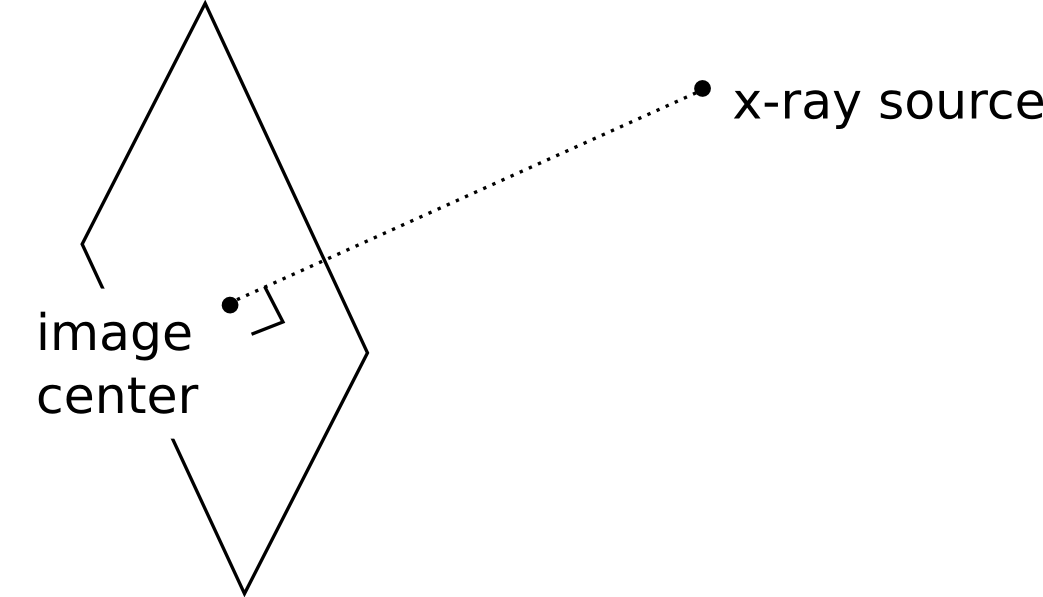
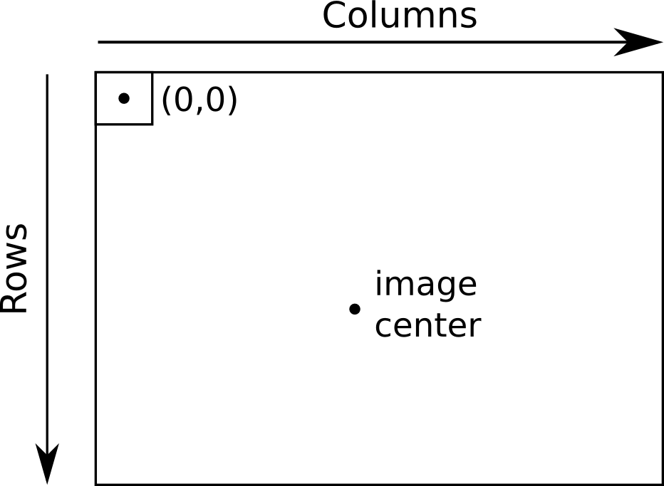
The image center is a pair of floating point numbers, in units of pixels. The first number is the column, the second number is the row. The first pixel of the image is considered to be coordinate (0,0). The image center does not need to lie within the bounds of the image.

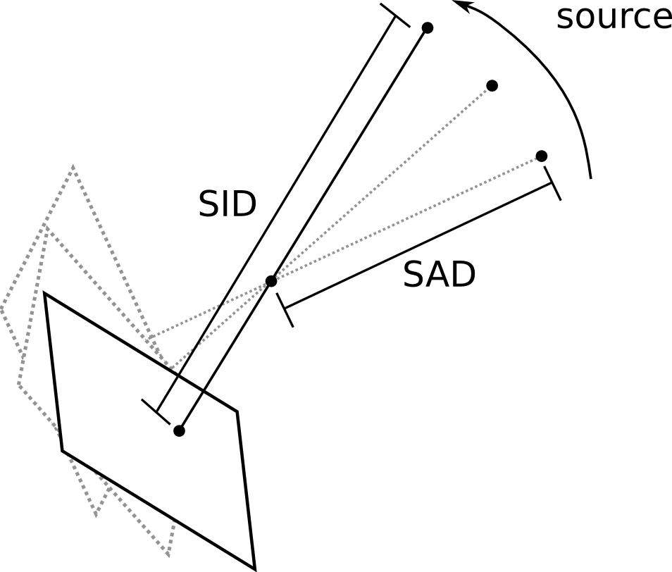
SID and SAD¶

The SID is the source-to-image distance, and the SAD is the source-to-axis distance. The SID is simply the 3D distance from the source to the image center. The SAD assumes a rotation axis, typically the axis of gantry rotation for cone-beam CT acquisition. The units for these quantities are millimeters.

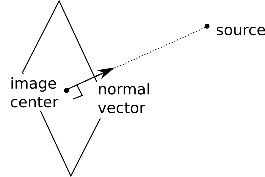
Normal vector¶

The normal vector refers to the world coordinate normal vector of the imaging device. It is the unit vector that points to the x-ray source as seen from the image center.

Projection matrix¶

The projection matrix is the 3 x 4 matrix the maps homogenous world coordinates into homogenous pixel coordinates.

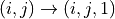
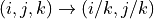
A homogenous world coordinate is a 4 x 1 vector. You can convert a 3D coordinate (x,y,z) into homogenous coordinates by appending a 1: (x,y,z,1). You can convert a homogenous coordinate (x,y,z,w) into a 3D coordinate by first dividing each element by w, and then taking the first three elements.

$(x,y,z) \rightarrow (x,y,z,1)$

$(x,y,z,w) \rightarrow (x/w,y/w,z/w)$

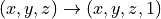
A similar procedure will convert 2D pixel coordinates to and from homogenous coordinates.

$(i,j) \rightarrow (i,j,1)$

$(i,j,k) \rightarrow (i/k,j/k)$

Let:

$\bf{i} := \left[\begin{array}{c} i \\ j \\ k \end{array} \right]$

$\bf{x} := \left[\begin{array}{c} x \\ y \\ z \\ w \end{array} \right]$

Suppose the imaging system is aligned with the world coordinates into a standard reference frame with the x-ray source at location (0,0,0), and the panel perpendicular to the z axis, at a distance defined by the SID. Suppose further that the pixel coordinate (0,0) is aligned with the image center, as shown here:

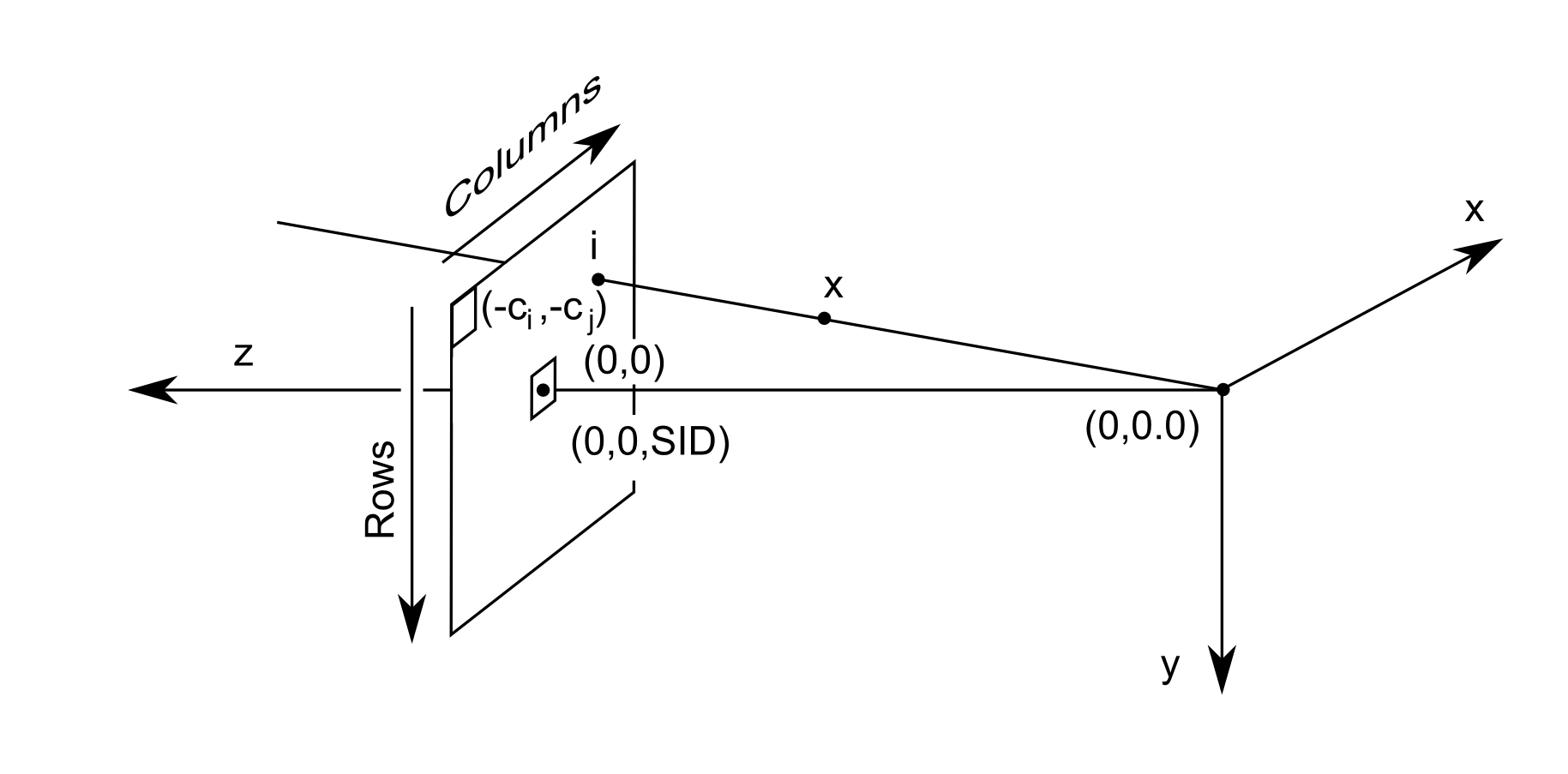
The mapping from world coordinates to image coordinates is therefore

$\bf{i} = K \bf{x}$

where K is the intrinsic matrix, defined as:

$K = \left[ \begin{array}{cccc} 1/\alpha & 0 & 0 & 0 \\ 0 & 1 / \beta & 0 & 0 \\ 0 & 0 & 1 / SID & 0 \end{array} \right]$

where alpha and beta are the pixel spacing for columns and rows. Note, that when you use K as defined above, you will need to add (c_i, c_j) later on to the final result. to get pixel coordinates.

In order to align the imaging system with the standard reference frame, we need to rotate and translate. This is called the extrinsic matrix, and is given by:

$C = \left[ \begin{array}{cccc} r_{11} & r_{12} & r_{13} & t_1 \\ r_{21} & r_{22} & r_{23} & t_2 \\ r_{31} & r_{32} & r_{33} & t_3 \\ 0 & 0 & 0 & 1 \end{array} \right]$

Here, R is the rotation, and t is the translation. First, the points are rotated, then a translation is added.

For example, if the imaging panel is perpendicular to the y axis (instead of the z axis) at distance SID, and the source was located at position (1000,0,0), we would have:

$C = \left[ \begin{array}{cccc} 1 & 0 & 0 & -1000 \\ 0 & 0 & -1 & 0 \\ 0 & 1 & 0 & 0 \\ 0 & 0 & 0 & 1 \end{array} \right]$

The composition of the intrinsic and entrinsic matrices is called the projection matrix. The extrinsic matrix rotates the world coordinate frame into a standard reference frame. Then, the intrinsic matrix flattens out the extra dimension.

$\bf{i} = K C \bf{x}$

$\left[\begin{array}{c} i \\ j \\ k \end{array} \right] = \left[ \begin{array}{cccc} 1/\alpha & 0 & 0 & 0 \\ 0 & 1 / \beta & 0 & 0 \\ 0 & 0 & SID & 0 \end{array} \right] \left[ \begin{array}{cccc} r_{11} & r_{12} & r_{13} & t_1 \\ r_{21} & r_{22} & r_{23} & t_2 \\ r_{31} & r_{32} & r_{33} & t_3 \\ 0 & 0 & 0 & 1 \end{array} \right] \left[\begin{array}{c} x \\ y \\ z \\ w \end{array} \right]$

Next, after computing (i,j,k), we convert from homogenous to pixel coordinates:

$(i,j,k) \rightarrow (i/k,j/k),$

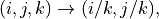
and finally, we correct for the image center:

$(i,j) = (i/k + c_i, j/k + c_j)$

Extrinsic and intrinsic matrices¶

These matrices are generated by the drr program, but aren’t used by the fdk program. They are included in the file format because they are sometimes useful for debugging.