Mutual information
The intensity  of a voxel located at coordinates
(
of a voxel located at coordinates
( ) within the fixed image
  is given
by:
is given
by:

and similarly, the intensity  of a voxel at coordinates
(
of a voxel at coordinates
( ) within the moving image
  is given
by:
is given
by:

We want to apply a coordinate transform
 to the moving image such that it
registers best with the fixed image
to the moving image such that it
registers best with the fixed image  . However, since
and could have been obtained from different
imaging modalities, we cannot simply minimize the error between
intensities
. However, since
and could have been obtained from different
imaging modalities, we cannot simply minimize the error between
intensities  and . Instead, we must attempt
to maximize the amount of information shared between the two
images. The statistical Mutual Information can therefore be
used as a similarity metric:
and . Instead, we must attempt
to maximize the amount of information shared between the two
images. The statistical Mutual Information can therefore be
used as a similarity metric:
(1)
which depends on the probability distributions of the voxel
intensities for the static and moving images. We now view
and as random variables with associated
probability distribution functions  and
and
 and joint probability
  . Note
that applying the spatial transformation
. Note
that applying the spatial transformation  to
will result in modification of . This
effect is implied with the notation
to
will result in modification of . This
effect is implied with the notation  .
Furthermore, if
.
Furthermore, if  results in voxels being
displaced outside of the image, will change.
Perhaps more importantly, if results in a
voxel being remapped to a location that falls between points on the
voxel grid, some form of interpolation must be employed to obtain
, which will modify . These effects are
implied with the notation
results in voxels being
displaced outside of the image, will change.
Perhaps more importantly, if results in a
voxel being remapped to a location that falls between points on the
voxel grid, some form of interpolation must be employed to obtain
, which will modify . These effects are
implied with the notation  .
.
The method of interpolation used to obtain given
is important both in terms of
execution speed and solution convergence. Here we will discuss the
Partial Volume Interpolation method proposed by Maes et. al.
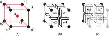
Figure 1(a) depicts the situation where  has displaced a voxel (red) to the center of a
neighborhood of 8 other voxels (black). The interpolation method divides the
volume defined by the 8-nearest neighbors (red) into 8 partial volumes (w1 -
w8) that all share the red voxel’s location as a common vertex Figure 1(b-c).
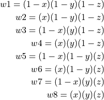
We can more formally define the 8 partial volumes as a function of
has displaced a voxel (red) to the center of a
neighborhood of 8 other voxels (black). The interpolation method divides the
volume defined by the 8-nearest neighbors (red) into 8 partial volumes (w1 -
w8) that all share the red voxel’s location as a common vertex Figure 1(b-c).
We can more formally define the 8 partial volumes as a function of
 :
:
(2)
Noting that

Once the partial volumes have been computed, they are placed into
the histograms of their corresponding voxels in the 8-neighborhood.
Partial volume  is placed into the histogram bin
associated with
is placed into the histogram bin
associated with  ,
,  with
with  , etc.
This method is used in computing both
and .
, etc.
This method is used in computing both
and .
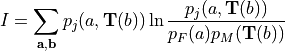
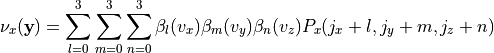
We now have a complete expression for the mutual information similarity metric, which we will use as a cost function that describes the quality of the registration.
(3)
We can attempt to achieve the optimal registration by maximizing this cost
function, which is achieved through modification of the coordinate
transformation applied to the moving image
. It is important to note that the could be any
type of conceivable coordinate transformation. For example,
could represent a set of affine transforms to be applied
to the moving image. Here, however, we will be focusing on a parametrically
defined nonrigid coordinate transformation. The transformation
is characterized by the displacement field
 , which defines how individual voxels within the moving image
should be displaced such that
, which defines how individual voxels within the moving image
should be displaced such that  and are
optimally registered. This displacement field is computed at every voxel
given the B-spline coefficients
and are
optimally registered. This displacement field is computed at every voxel
given the B-spline coefficients  defined for the sparse array of
control-points:
defined for the sparse array of
control-points:
(4)
where ( ) form the indices of the 64 control points
in the immediate vicinity of a voxel located at
(). Note, (
) form the indices of the 64 control points
in the immediate vicinity of a voxel located at
(). Note, ( ) forms the
voxel’s offsets within the region bound by the 8 control-points in
the immediate vicinity of the voxel. For simplicity, we refer to
such a region as a tile.
) forms the
voxel’s offsets within the region bound by the 8 control-points in
the immediate vicinity of the voxel. For simplicity, we refer to
such a region as a tile.
Having defined the coordinate transformation
in terms of the B-spline
coefficients , it is becomes apparent that the mutual
information may be maximized through optimization of .
If this is to be accomplished via the method of gradient descent,
an analytic expression for the gradient
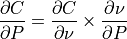
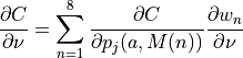
 must be derived. The chain rule
is employed to separate the expression into two partial derivatives
with the first being dependent on the similarity metric employed
and the second on the type of transform employed:
must be derived. The chain rule
is employed to separate the expression into two partial derivatives
with the first being dependent on the similarity metric employed
and the second on the type of transform employed:
(5)
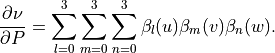
where the second term is easily obtained by taking the derivative
of (4) with respect to :
Referring again to the first term of (5), it is
important to realize that  and
and  are coupled
through the probability distribution
are coupled
through the probability distribution  and are
therefore directly affected by the 8 neighborhood partial volume
interpolation. This becomes further apparent when
and are
therefore directly affected by the 8 neighborhood partial volume
interpolation. This becomes further apparent when
 is further decomposed:
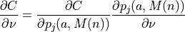
(6)
where the first term may be found by taking the derivative of
(3) with respect to the joint distribution :
(7)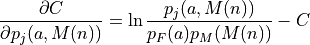
see {A}.
The second term, 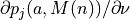 ,
describes how the joint distribution changes with the vector field.
Explicitly stated, a displacement vector locally transforms the
coordinates of a voxel in the moving image such that:
,
describes how the joint distribution changes with the vector field.
Explicitly stated, a displacement vector locally transforms the
coordinates of a voxel in the moving image such that:

From Figure fig:pv8 it becomes immediately apparent that as the vector field is
modified the partial volumes -  to be inserted into
the moving and joint histograms
to be inserted into
the moving and joint histograms  and will change in
size. Consequently,
and will change in
size. Consequently,  can be
found for
can be
found for  by taking the derivative of (2)
with respect to each of the Cartesian directions.
by taking the derivative of (2)
with respect to each of the Cartesian directions.
Therefore, as prescribed by (6), computing  at a given voxel in involves first cycling through the
8-bins corresponding to the 8 nearest neighbors used during the partial volume
interpolation and computing
at a given voxel in involves first cycling through the
8-bins corresponding to the 8 nearest neighbors used during the partial volume
interpolation and computing  for each, which
is scalar and therefore the same for all Cartesian directions. The 8
values are each weighted by one
for each, which
is scalar and therefore the same for all Cartesian directions. The 8
values are each weighted by one
 . Finally, once this process has been
completed for all 8 bins, the resulting
values is assimilated into the sparse coefficient array by way of
(5). Once this is completed for all voxels, the next optimizer
iteration begins and the process is repeated with a modified coefficient array
.
. Finally, once this process has been
completed for all 8 bins, the resulting
values is assimilated into the sparse coefficient array by way of
(5). Once this is completed for all voxels, the next optimizer
iteration begins and the process is repeated with a modified coefficient array
.
NOTE
It is important to note that if all 8 histograms associated with
the neighborhood are equal, the value of
 . This is a direct result
of
. This is a direct result
of

and similarly for the  - and
- and  -directions. However, when
the 8 histograms within the neighborhood are not equal, this will result in the
gradient
-directions. However, when
the 8 histograms within the neighborhood are not equal, this will result in the
gradient  being “pulled” in the Cartesian
direction of voxels associated with large ,
which is desirable when attempting to maximize MI.
being “pulled” in the Cartesian
direction of voxels associated with large ,
which is desirable when attempting to maximize MI.