Regularization¶

The plastimatch B-spline registration algorithm features a second derivative regularization term, which can be computed either analytically or numerically. Regularization usually improves both accuracy and vector field smoothness, so you are encouraged to try it on your problem.

The general form is given as:

$c = c_{IM} + \lambda c_{RM}$

where $c$ is the registration cost that is being optimized. The cost has two terms: an intensity metric term ( $c_{IM}$ ) and a regularization metric term ( $c_{RM}$ ). The intensity metric penalizes the images that do not match well, and the regularization term penalizes vector fields that are not smooth. The term $\lambda$ is used to trade off between image matching and vector field smoothness. Typical values of $\lambda$ range between 0.005 and 0.1.

The regularization term used in plastimatch is the square of the vector field second derivative. For a vector field $u = (u_x, u_y, u_z)$ , the regularization term is given as:

$c_{RM} = \int c_{RM,x} + c_{RM,y} + c_{RM,z}$

where

$c_{RM,x} = \left[ \left( \frac{\partial u^2_x}{\partial x^2} \right)^2 + \left( \frac{\partial u^2_x}{\partial y^2} \right)^2 + \left( \frac{\partial u^2_x}{\partial z^2} \right)^2 \right] + 2 \times \left[ \left( \frac{\partial u^2_x}{\partial x \partial y} \right)^2 + \left( \frac{\partial u^2_x}{\partial x \partial z} \right)^2 + \left( \frac{\partial u^2_x}{\partial y \partial z} \right)^2 \right].$

The integration is generally defined to be performed over the domain of the fixed image.

Analytic regularization¶

The default choice is to perform analytic regularization. Analytic regularization is generally preferred over numeric regularization becuase it runs much faster than numeric regularization, and gives similar results. However, it should be noted that the regularization is performed over all B-spline tiles that overlap the fixed image, which is a slightly larger domain of integration than the numeric methods use.

The method works tile by tile. Each tile is influenced by 64 control points, which are formed into a vector $v$ . Or to be more precise, there are 192 control points, three in each direction, which are formed into three vectors: $v_x$ , $v_y$ , and $v_z$ . The smoothness is computed directly from the control points using a 64x64 matrix $K$ , as a quadratic form:

$c_{RM} = v_x' K v_x + v_y' K v_y + v_z' K v_z.$

The matrix $K$ is precomputed, and can be reused for each tile. The results are then numerically integrated tile-by-tile over the fixed image.

Numeric regularization (flavor a)¶

Numeric regularization flavor “a” uses finite differencing to compute the derivatives, and then numerically integrates these result over all voxels.

Numeric regularization (flavor d)¶

Numeric regularization flavor “d” is a mixed analytic-numeric method. The derivatives are computed analytically at each voxel, and then numerically integrated over all voxels.

Stiffness images¶

If desired, a stiffness image can be used to perform voxel-specific regularization. At this time, this is supported only for numeric regularization.

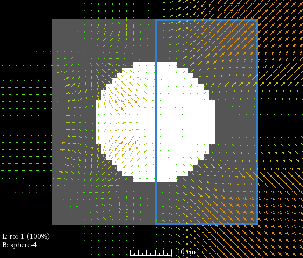
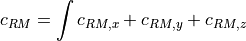
As an example, consider a registration with a sphere as the fixed image, and a cube as the moving image. A stiffness image has been created with stiffness of one in the right side of the image (outlined in blue), and a stiffness of zero elsewhere:

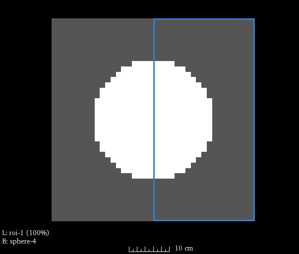
The registration command file is specified to use a stiffness map, with regularization lambda of 2.5. The penalty in the right side of the image is therefore 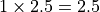$1 \times 2.5 = 2.5$ .:

[GLOBAL]
fixed=cube.mha
moving=sphere.mha
fixed_stiffness=stiffness_image.mha

[STAGE]
xform=bspline
regularization=numeric
regularization_lambda=2.5

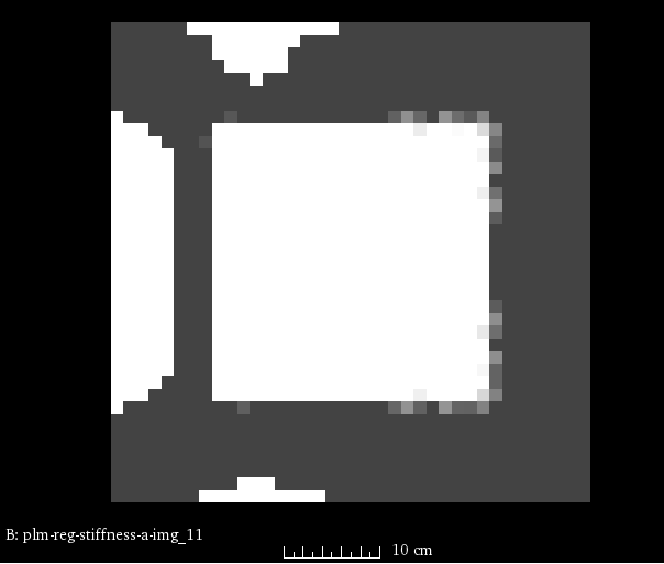
The result is an image with uneven regularization: